library(tidyverse) # for data manipulation and plots, and more besides
library(ggfortify) # this is useful for diagnostics
library(palmerpenguins) # for the palmer penguin data8 One-way ANOVA
For this chapter you will find it useful to have this RStudio project folder if you wish to follow along and/or see how a complete script might look. Once the folder is downloaded, unzip it if you need to, put it somewhere sensible on your laptop then open the project from within RStudio using File/Open Project, whereupon you navigate to the project folder and then click on the .Rproj file.
8.1 Introduction
In this exercise we will carry out a method of analysis known as ANOVA - this is what is commonly used when you have one or more categorical variables, such as species, sex and so on, and a numerical response variable such as body mass and you want to know if there is a difference in the response variable between when the levels of the factors take different values.
A one-way ANOVA is used where where we have one categorical variable with three or more levels (you could also use it where there are just two levels, but we use a t-test for that). For example if you want to see if a captive bird species prefers red, green or blue food pellets, then the factor would be be food colour, and three levels of that would be the three colours.
A two-way ANOVA is used where we have two categorical variables, each of which has at least two levels. (Even if both have two levels, we still call it a two-way ANOVA. There is no such thing as a two-way t-test!). So, sticking with the captive birds, if were interested in whether they had a preference for colour (red, blue, green) and/or shape (round, square) of food pellets, then we could use a two way ANOVA to investigae the data, where the two factors or ‘ways’ would be food colour and food shape, with food colour having three levels (red, blue and green) and food shape having two levels (round and square).
ANOVAs involving three ways or more (the horror, the horror!) are rarely used since their interpretation is in practice difficult due to the multiplicity of possible so-called ‘interaction’ effects that commonly arise, whereby the impact on the output of the levels of one factor depend on the values of the levels of one or more other factors. Best avoided!
ANOVAs, whatever their flavour (one way, two way, repeated measures, ANCOVA etc) are examples of parametric tests. That is, they can only be used if the data at least approximately meet certain requirements such as equal variance across the data sets, normality of residuals etc. At the very least, the data should be numerical and not ordinal. Hence whenever we think of using an ANOVA we need to check that these requirements are at least approximately met. If they are not, then we may choose to turn to non-parametric alternatives.
A non-parametric alternative to a one-way ANOVAs is commonly used, especially for studies that involve ordinal data such as Likert-type outputs from surveys. It is called a Kruskal-Wallis test.
8.2 One-way ANOVA: Female penguin data from the palmerpenguins package
In the following, we show how a one-way ANOVA might be carried out on a set of data on female penguins, where we have a numerical output such as body mass, and one categorical variable which is species (three levels: Adelie, Gentoo and Chinstrap). If we were interested in whether there was a difference in the output across the levels of species, then a one-way ANOVA might well be suitable.
Let’s ask the question: do the body weights differ between females of the different species?
There is just one factor here, species, and it has more than two levels - the three different species - and the reponse variable is numeric, so it is highly likely that the appropriate test to answer this question is a one-way ANOVA. ‘One way’ because there is one factor, and ‘ANOVA’ (instead of t-test) because there are more than two levels.
8.2.1 Null hypothesis
Pretty much all of the commonly used statistics tests are asking the question: what is the probability that you would have got this data, or more extreme data, if the null hypothesis were true? Their job is to calculate that probability, which is called a p-value. There is a lot more besides, but what this means is that in carrying out any of these tests we at least need to have a hypothesis in mind and its corresponding null hypothesis. The null, remember, is typically the ‘nothing going on’, there is no effect, no difference scenario.
So in this case, a suitable null hypothesis would be that there is no difference in body mass between the females of the different penguin species.
To see if there is evidence from the data to reject this null, we will follow a sequence of steps that will be common to many analyses:
- get the data
- clean/prepare the data
- summarise the data
- plot the data
- construct the model using whatever test is appropriate, in this case a one-way ANOVA
- check whether the model is valid
- inspect the model output
- reject or fail to reject the null hypothesis
- if we reject the null, carry out post-hoc tests
- (maybe) simplify the model and redo the analysis
For the penguin data, getting it was easy as it came with the palmerpenguins package.
8.2.2 A first look at the data
First we need to get the data! The data set we want comes as part of the palmerpenguins package, so we load that here along wih the tidyverse and ggfortify packages, the latter becuase it has the function autoplot() which we will use for diagnostics.
Load packages
The palmerpenguins package comes with two in-built data sets on penguins. The simplest of them is called penguins and is the one we will use in this exercise:
glimpse(penguins)Rows: 344
Columns: 8
$ species <fct> Adelie, Adelie, Adelie, Adelie, Adelie, Adelie, Adel…
$ island <fct> Torgersen, Torgersen, Torgersen, Torgersen, Torgerse…
$ bill_length_mm <dbl> 39.1, 39.5, 40.3, NA, 36.7, 39.3, 38.9, 39.2, 34.1, …
$ bill_depth_mm <dbl> 18.7, 17.4, 18.0, NA, 19.3, 20.6, 17.8, 19.6, 18.1, …
$ flipper_length_mm <int> 181, 186, 195, NA, 193, 190, 181, 195, 193, 190, 186…
$ body_mass_g <int> 3750, 3800, 3250, NA, 3450, 3650, 3625, 4675, 3475, …
$ sex <fct> male, female, female, NA, female, male, female, male…
$ year <int> 2007, 2007, 2007, 2007, 2007, 2007, 2007, 2007, 2007…8.2.3 Filter and clean the data
With any data set there is normally some sort of cleaning or preparation that you have to do before you can plot or analyse it. That may mean narrowing down to certain species, dates, sites etc, transforming the data in some way or dealing with missing data.
To prepare the penguin data for our purposes here, we narrow the full data set down to just the females, using the filter() function, and then make sure there are no lines with missing values, using drop_na(). We save this cleaned data set in an object called females.
females <- penguins |>
  filter(sex == "female") |>
  drop_na()
8.2.4 Summary - group by species
Here we use the famliar group_by() and summarise() construction to find the mean body mass for the females of each species. We also calculate the standard error of those means and the number of individuals in each group.
females.summary <- females |>
  group_by(species) |>
  summarise(n = n(),
            mean.mass_f = mean(body_mass_g),
            sd.mass_f = sd(body_mass_g),
            se.mass_f = sd.mass_f/sqrt(n()))
females.summary
# A tibble: 3 × 5
species n mean.mass_f sd.mass_f se.mass_f
<fct> <int> <dbl> <dbl> <dbl>
1 Adelie 73 3369. 269. 31.5
2 Chinstrap 34 3527. 285. 48.9
3 Gentoo 58 4680. 282. 37.0We should inspect this summary table and see what we already think about whether the null hypothesis is likely to be rejected, or not.
Next we should plot the data, using our favourite plot type. Whatever the type, it would ideally, in some way, show the central value and spread of the data as well as the sample size. Here we use a simple box plot (it’s OK, but not ideal!):
8.2.5 Plot the data
females  |>
  ggplot(aes(x=species, y = body_mass_g)) +
  geom_boxplot(fill = "#9ebcda") +  # pick your favourite colour from https://colorbrewer2.org/
  labs(x = "Species",
       y = "Body mass (g)") +
  theme_bw()
Note
The box-plot shown above is OK, but it only crudely shows the distribution of the data annd it does not show the sample size. Consider this alternative plot. More code is needed to make it, but it gives you an idea of what can be done with ggplot. The plot shows mean values and standard devation error bars above a cloud of the actual data points for each species, where some sideways jitter has been added to these so that they do not lie on top of one another.
Unlike the box plot, this plot gives you a clear sense of the sample sizes and of the actual distribution of data within each sample.
females  |>
  ggplot(aes(x=species, y = body_mass_g)) +
  geom_jitter(colour = "#9ebcda", fill = "#9ebcda", width = 0.2, alpha = 0.5) +  # pick your favourite colour from https://colorbrewer2.org/
  geom_errorbar(data = females.summary,
                inherit.aes = FALSE,
                aes(x = species, ymin = mean.mass_f - sd.mass_f, ymax = mean.mass_f + sd.mass_f ),
                colour = "gray50",
                width = 0) +
  geom_point(data = females.summary, aes(x = species, y = mean.mass_f), colour = "gray40", size = 3) +
  labs(x = "Species",
       y = "Body mass (g)") +
  theme_bw()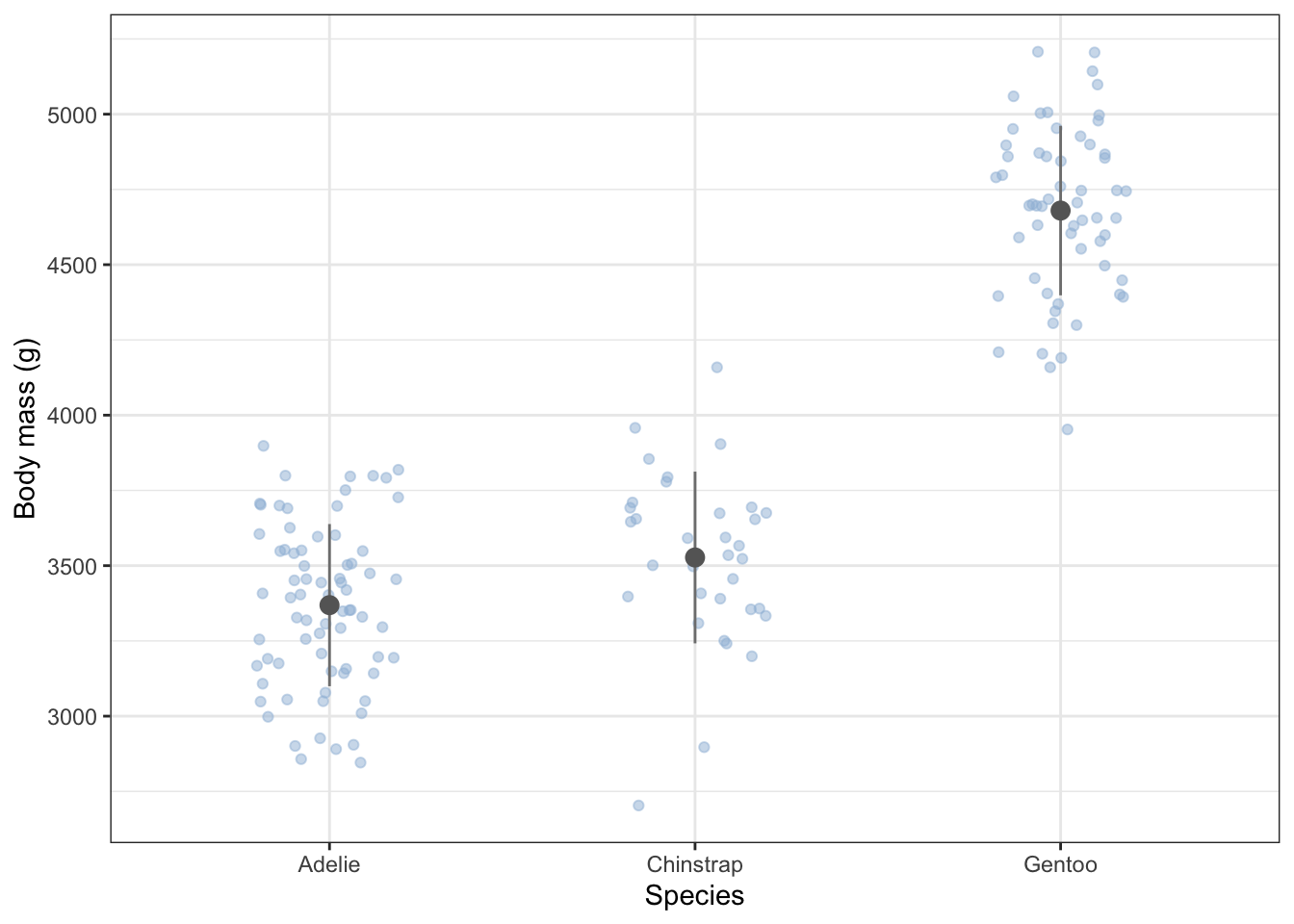
From the summary table and the plot, what do you think? Do the masses differ between the species?
8.2.6 Statistical analysis
By now you probably have a good idea what the answer is as to our question but now we will move on to the actual statistics test, in this case a one-way ANOVA followed by post-hoc tests.
An ANOVA is one variant of a range of anlysis techniques known as ‘linear models’. If you were to look under the hood, you would see that mathematics behind it is exactly the same as that behind linear regression, which we use when we have a continuous explanatory variable and where we fit straight lines onto a scatter plot. An ANOVA is just the same except that the explanatory variable is categorical. Thus it should be no surprise that the ANOVA is carried out in R in exactly the same way as linear regression would be:
First, we use the lm() function to construct a linear model of the data:
8.2.6.1 Construct the ANOVA model
females.model <- lm(body_mass_g ~ species, data = females)Here the lm() function has done all the maths of the ANOVA, and we have saved the results of that in an object called females.model. Note the use of the formula body_mass_g ~ species as the first argument of the lm() function, where this means ‘body mass as a function of species’.
8.2.6.2 Check if the model is valid.
All linear models are only valid if the data meet a number of criteria. Chief among these for an ANOVA is that the spread of the data should be roughly the same in each subset, and that the data within each subset should be normally distributed around their respective mean values. Only if these conditions are at least approximately met can we just go on and trust the output of the model. If they are not, we need to transform the data in some way until they are, or use a different test. A commonly used non-parametric alternative to the one-way ANOVA is the Kruskal-Wallis test.
There are various ways we can find out whether these conditions are met. A useful one is to do it graphically, and a handy way to do that is to use the autoplot() function from the ggfortify package. Let’s do it:
autoplot(females.model) + theme_bw()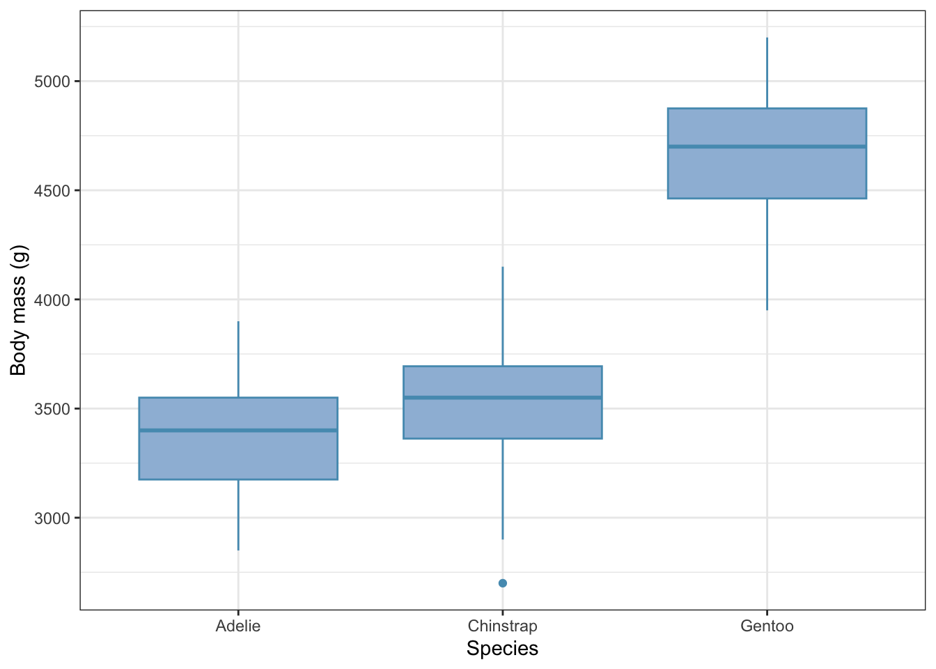
All four graphs presented here tell us something about the validity or not of our model. Here we will just focus on the upper two:
top-left: this shows the spread of the residual masses (difference between an individual’s mass and the mean mass for it’s species) for each species. We see that the spread of these values is about the same for all three species. Check!
top-right: this is a
quantile-quantileplot, often referred to as a qq-plot. This compares the distribution of the residuals for each species with those of a normal distribution. If the residuals are normally distributed, we will get a straight line. If not, we won’t. To get an idea of what qq-plots, histograms and box-plots look like for data that definitely are not normally distriuted, see this useful summary. In our case, there is a hint of a curve, but this qq-plot is really a pretty good approximation to linear for a real data set. No such data is ever perfectly normally distributed, so the best we are looking for, in practice, is something approximating a straight line, often with some raggedness at either end. So, check again!
On both counts, we are good to go: we can reasonably trust the output of the ANOVA.
So what is this output? We find this in two, sometimes three, steps.
8.2.6.3 Inspect the model
The overall picture
First, we use the anova() function
anova(females.model)Analysis of Variance Table
Response: body_mass_g
Df Sum Sq Mean Sq F value Pr(>F)
species 2 60350016 30175008 393 <2e-16 ***
Residuals 162 12430757 76733
---
Signif. codes: 0 '***' 0.001 '**' 0.01 '*' 0.05 '.' 0.1 ' ' 1This gives us an overview of all the data and asks the question: how likely is it that you would have got your data if species made no difference to body mass. There are three things to note:
the test statistic, here called an F-value. This is a number calculated from the data. Roughly speaking, it is the ratio of the spread of values (aka variance) between the subgroups to that within the subgroups If the validity criteria for the test have been met by the data, then this has a known distribution. The bigger the F-value, the more likely it is that the null will be rejected.
the
degrees of freedom, here denoted as Df and listed in the first column. These are the number of independent pieces of information in the data, which here relates to how many species and how many penguins were included in the study.the p-value, which is the probability of getting an F value as big as or bigger than the one actually found, if the null hypothesis were true. This is is the number listed at the right as Pr(>F).
The F value here is huge and the p-value is tiny, so tiny that it is essentially zero. Thus we can confidently reject the null hypothesis and assert that there is evidence from the data that body mass of females differs between at least one pair of species. Which two, or between all of them, and by how much we don’t yet know. This first step just tells us whether there is some difference somewhere. If there were no evidence of any difference we would stop the analysis right here.
But there is a difference in this case, so we continue.
The detailed picture
If we are interested in the differences between a control level and all the other levels, then the summary() analysis outlined in the next section is what we need. If on the other hand all we are interested in is whether there are any statistically significant pairwise differences that are big enough to be important, then we can skip this section and go on to Section 8.2.7.
If we do want know differences relativ to some control, we use the summary() function:
summary(females.model)
Call:
lm(formula = body_mass_g ~ species, data = females)

Residuals:
   Min     1Q Median     3Q    Max
-827.2 -193.8   20.3  181.2  622.8

Coefficients:
                 Estimate Std. Error t value Pr(>|t|)
(Intercept)        3368.8       32.4  103.91   <2e-16 ***
speciesChinstrap    158.4       57.5    2.75   0.0066 **
speciesGentoo      1310.9       48.7   26.90   <2e-16 ***
---
Signif. codes:  0 '***' 0.001 '**' 0.01 '*' 0.05 '.' 0.1 ' ' 1

Residual standard error: 277 on 162 degrees of freedom
Multiple R-squared:  0.829, Adjusted R-squared:  0.827
F-statistic:  393 on 2 and 162 DF,  p-value: <2e-16
There is a lot in ths output, so let’s just consider the coefficient table, to begin with. Focus first on the top left value, in the Estimate column. This tells us the mean body mass of the reference or ‘Intercept’ species. In this case that is ‘Adelie’, purely because ‘Adelie’ comes alphabetically before the other two species names, ‘Chinstrap’ and ‘Gentoo’. By default, R will always order levels of a factor alpabetically. This is often a nuisance, and with many data sets we have to tell R to reorder the levels the way we want them, but here the order is OK.
So, the mean mass of female Adelie penguins in our sample is 3368 g. Cross check that with your initial summary table and the box plot. What about the other two species? Here’s the thing: for all rows except the first in the Estimate column we are not given the absolute value but the difference between their respective mean values and the reference mean in the first, ‘Intercept’ row.
Thus, we are being told that Chinstrap females in the sample have a mean body mass that is 158.37 g heavier than that of Adelie females, so that their mean body mass is 3368.84 + 158.37 = 3527.27g. Again, cross check that with your summary table and the box plot. Is it right?
What about Gentoo females? Were they heavier than Adelie penguins, and if so, by how much? What was their mean body mass.
Why doesn’t summary() just tell us the actual body masses instead for all three species instead of doing it in this round about way? The reason is that ANOVA is concerned with detecting evidence of difference. This is why we are being told what the differences are between each of the levels and one reference level, which here is Adelie.
Are those differences significant? We use the right hand p-value column to determine that. Look in the rows for Chinstrap and Gentoo penguins. In both cases the p values are much less than 0.05. This is telling us that in both cases there is evidence that females of these species are significantly heavier than those of the Adelie species.
Note that we have only been told, so far, about the magnitude and significance of differences between all the levels and the reference level. We are not told the significance of any difference between any other pair of levels. So in particular, the ANOVA does not tell us whether there is a significant difference between the masses of Chinstrap and Gentoo females (although we may have a good idea what the answer is, from our initial summary table and plot).
To find the answer to that, we do post-hoc tests:
8.2.7 Post-hoc tests.
A final step of most ANOVA analyses is to perform so-called post-hoc (‘after the fact’) tests which make pairwise comparisons between all possible pairs of levels. These tell us what the differences are between those pairs and whether these differences are significant. Whatever method is used for this, it needs to take account of the danger of making Type-one errors that arises when multiple pair-wise tests are done. The study-wide Type-One error rate needs to be controlled and kept below 0.05 (or whatver significance level you have set).
A commonly used way to do this is to use the emmeans package
library(emmeans)
emm <- emmeans(females.model, ~ species)
pairs(emm, adjust = "tukey")
contrast estimate SE df t.ratio p.value
Adelie - Chinstrap -158 57.5 162 -2.750 0.0180
Adelie - Gentoo -1311 48.7 162 -26.900 <0.0001
Chinstrap - Gentoo -1153 59.8 162 -19.260 <0.0001
P value adjustment: tukey method for comparing a family of 3 estimates THis gives all pairwise comparisons between groups with Tukey-adjusted p-values (equivalent to Tukey’s HSD, but more flexible) to keep the study-wide error rate down despite multiple pairwise testing.
In each row of the estimate column of the output we are given the difference between the mean masses of the females of the two species named in the contrast column, where the mean of the second named species is subtracted from the mean of the first. A negative difference means that the mean of the second named species is greater than that of the first. So, we see that Gentoo females in the sample were on average 1310.9 g heavier than Adelie females.
Compare these differences with your initial summary table and your box plot. Do they agree? They should!
The right-hand column ‘p.value’ tells us whether these difference are significant. If the p values are less than 0.05 then they are, at the 5% significance level. In this case they all are. The p values are so tiny for the differences between Gentoo and the other two species that their exact values are not reported. We are just told that each is less than 0.0001 That is enought to tell us that they are much less than 0.05 which is all we need to know.
8.2.8 Reporting the Result.
We try to use plain English to report our results, while still telling the reader what test was used and the key outputs of the test. Try to report the name of the test, the test statistic, the degrees of freedom, the p-value and, crucially, in some way indicate the effect size. A good way to indicate the estimated value, the precision of that estimate and the significance all in one is to report the confidence interval. If the p-value is really small then it is common to report it as p<0.01, or p<0.001. No one cares if it is a billionth or a squillionth. It just matters that is t is really small, if that is the case. If it is only just below 0.05, then I would report it in full, so we might write p = 0.018. If p > 0.05 then conventiallly it is not reported, except to say p > 0.05.
In this case, we might say something like:
We find evidence that there is a difference between the body masses of females of the penguin species Adelie, Chinstrap and Gentoo (ANOVA, df = 2, 162, F = 393, p < 0.001). In particular Gentoo are more than 1 kg heavier than the other two (p< 0.001) while the difference between Chinstrap and Adelie is smaller, at 158 ± (SE)58 g , but still significant (p = 0.018).
8.3 Summary of the ANOVA workflow
In summary, once you have created the ANOVA object females.model using lm(), the sequence of steps is:
- Check assumptions / diagnostics using
autoplot(females.model) - Test the overall effect of group using
anova(females.model) - If significant (or if you have planned comparisons with a reference or control level), examine the model coefficients and/or estimated means using
summary(females.model) - Do post-hoc pairwise comparisons using
emmeans()in the manner shown in Section 8.2.7 - Report effect sizes and/or confidence intervals