24 Error bars
24.1 What are error bars for?
Error bars perform two main functions. One of these is a descriptive function, to give readers an idea of the spread of values within a data set, and thus of the spread within the population from which the data have been drawn. The other is inferential, to enable readers to make inferences from a data set, for example to enable them to determine whether two data sets are plausibly drawn from the same population. These two functions are quite different.
24.2 Descriptive error bars
We could indicate the spread of values of a data set using the range or the standard deviation. Range error bars go from the highest to the lowest value in the data set, while standard deviation \(SD\) is calculated using the formula
\[ SD=\sqrt{\frac{\sum_{i=1}^n\left(y_i-\bar{y}\right)^2}{n-1}} \] where the sum \(\sum\) is of the squared differences between the sample values \(y_i\) and the sample mean \(\bar{y}\), over all \(n\) data points in the sample. \(SD\) can be thought of, roughly speaking, as the average deviation of data points in a sample from the mean of the sample.
For a sample of data points that are approximately normally distributed around their mean, about two thirds of the data set will lie within one standard deviation either side of the mean while about 95% of the data set will lie within about two standard deviations of the mean. Thus, only about 5% of all such data are more than two SDs away from the mean, so if a new data point is more than 2 SD from the mean, you can regard it as unusual.
The standard deviation of a sample will in general be approximately equal to the population standard deviation \(\sigma\) and so can be used as an estimate for it. It gives an idea of the spread of values within the population, and also of the likely spread of values in any other sample taken from that population. If we take sample after sample from the population we would get a different sample standard deviation every time but there would be no systematic reduction in standard deviation for larger sample sizes. Instead, these values would dot around the true value for the population, but with less and less fluctuation for larger sample sizes: the larger the sample size, the closer the sample standard deviation is likely to be to the population standard deviation.
However, the SD of the experimental results will approximate to \(\sigma\), whether n is large or small. Like M, SD does not change systematically as n changes, and we can use SD as our best estimate of the unknown \(\sigma\), whatever the value of n.
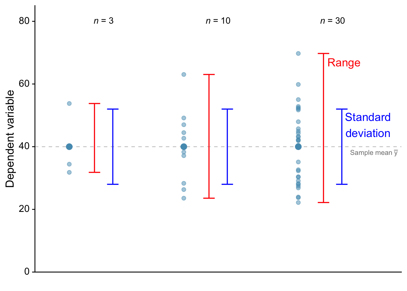
Figure 24.1 above shows means with error bars for three cases of sample size: n = 3, n = 10, and n = 30. The small black dots are data points and the large black dots represent the sample means. The red bars against each sample show range, while the blue bars show standard deviation (SD). The mean \(\bar{y}\) and SD have been made to be the same for every case here, but notice how much the range increases with \(n\). This happens because larger samples are more likely to capture extreme values within a population than small samples. Note also that although the range error bars encompass all of the experimental results, they do not necessarily cover all the results that could possibly occur. The population may include larger or smaller individuals than those included in the sample.
SD error bars include about two thirds of the sample, and 2 x SD error bars would encompass roughly 95% of the sample.
24.3 Inferential Error Bars
24.3.1 The standard error
Often in biology and ecology one wants to know if two or more samples of data provide convincing evidence that the populations from which they have been drawn are different. One wants to infer from what we know to be the case for the samples, (that they have this or that sample means and standard deviations), to a statement about their respective populations. To indicate this in a figure, we can use either of two other types of error bar: the standard error of the mean or the confidence interval.
If we know these then we know, roughly speaking, the range of values within which the means of the whole populations from which we drew our samples might plausibly lie, and thus whether we can reasonably reject the claim that there is no difference between these, so that the samples must have effectively been drawn from the same population.
Supposing, in a hypothetical world, you could take sample after sample from a population, each sample presumed to be independent of all the others, and all of size n replicates. Each would most likely have a different mean from all the others, but the collection of sample means would be normally distributed around the true population mean. The ‘standard error of the mean’ is the standard deviation of this distribution, which is often referred to as the sampling distribution. This is the ‘typical’ or roughly speaking the average deviation between a randomly chosen sample mean and the true, population mean. It is given by
\[SE = \frac{SD}{\sqrt{n}} \]
where SD is the standard deviation of an individual sample and n is the sample size. Thus, unlike the standard deviation of a sample, the standard error of the mean of the samples does systematically get smaller as the sample size n increases. This is another way of saying that, the larger a sample is, the closer its mean is likely to be to the population mean. Another thing to notice is that the SE is proportional to the SD, which is to say that sample means are more likely to be a close approximation to the population mean if the spread of values within the population, and thus the sample, is small. Smaller SD means smaller SE. Who knew?
24.3.2 The confidence interval
The confidence interval is an inferential tool, like the standard error and unlike the standard deviation. That means, we repeat, that it does not so much indicate the spread of values in a sample or estimate the spread of values in a population - that is what the standard deviation does. Instead, like the standard error, it indicates the range of values within which the true mean of a population might plausibly lie.
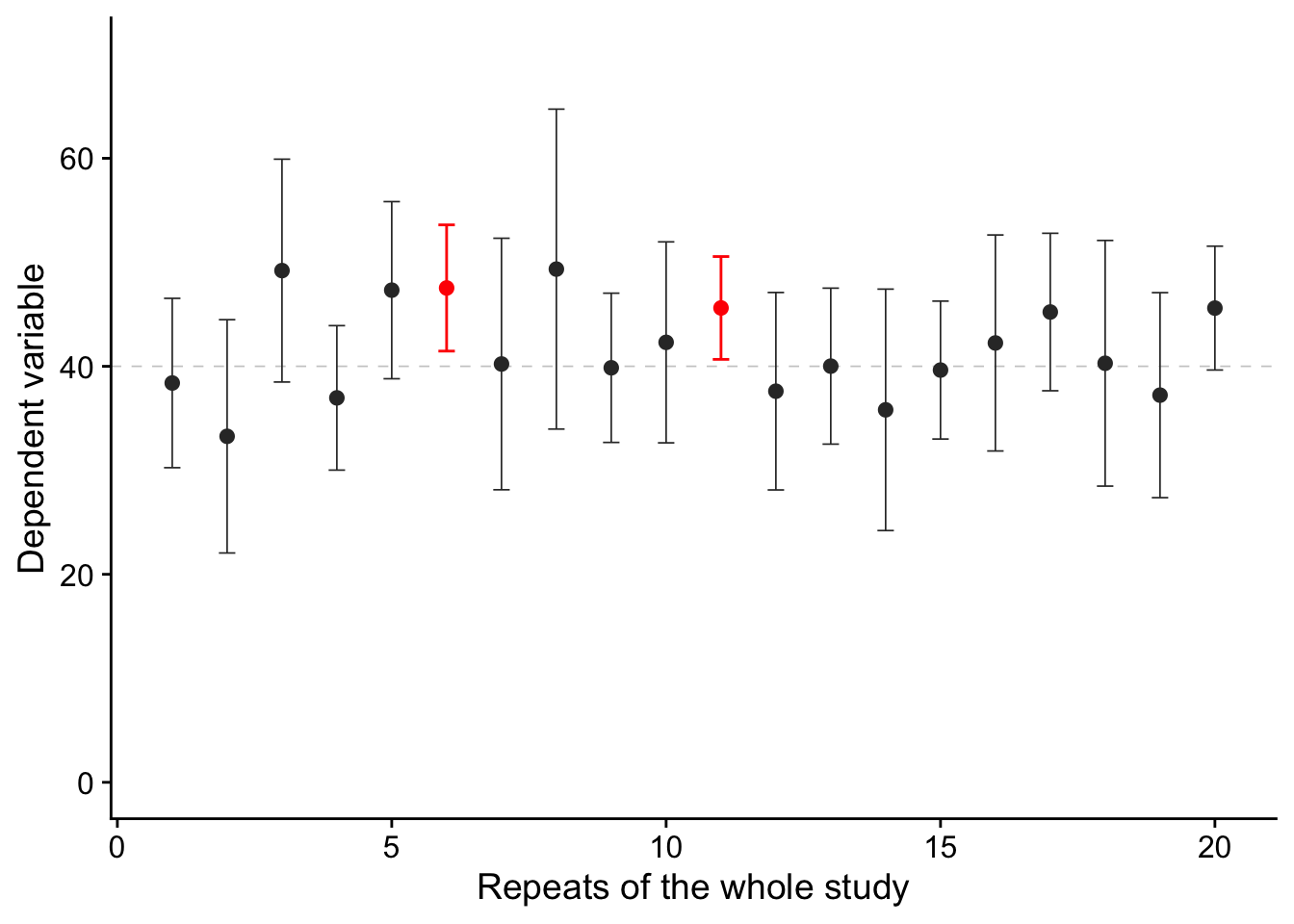
What do we mean by plausibly? Well, we could mean, say, that we are confident that the true mean would be in the interval 95% of the time if we calculated it again and again, as in Figure 24.2.
Confidence intervals around an estimated value tell us several things:
- They tell us the estimated value - this is usually, but not always in the centre of the interval.
- They tell us how precise the estimate is - we get this from the width of the interval, from the lower bound to the upper bound.
- They tell us whether our estimates are significantly different from zero, or any other threshold of interest. Any value within the interval is a plausible value for whatever we are estimating so if the interval encompasses zero then whatever we are estimating could be zero. Put another way, the confidence interval tells us whether our data provide evidence to reject the null hypothesis that our estimate is zero. If zero is in the confidence interval then they don’t provide this evidence but if it is, then they do.
24.3.3 How to interpret figures
| ID | Estimate | p-value | LB | UB |
|---|---|---|---|---|
| B-A | -0.531 | 0.4822 | -2.049 | 0.987 |
| C-B | 1.675 | 0.0318 | 0.155 | 3.196 |
| C-A | 1.144 | 0.0807 | -0.147 | 2.435 |
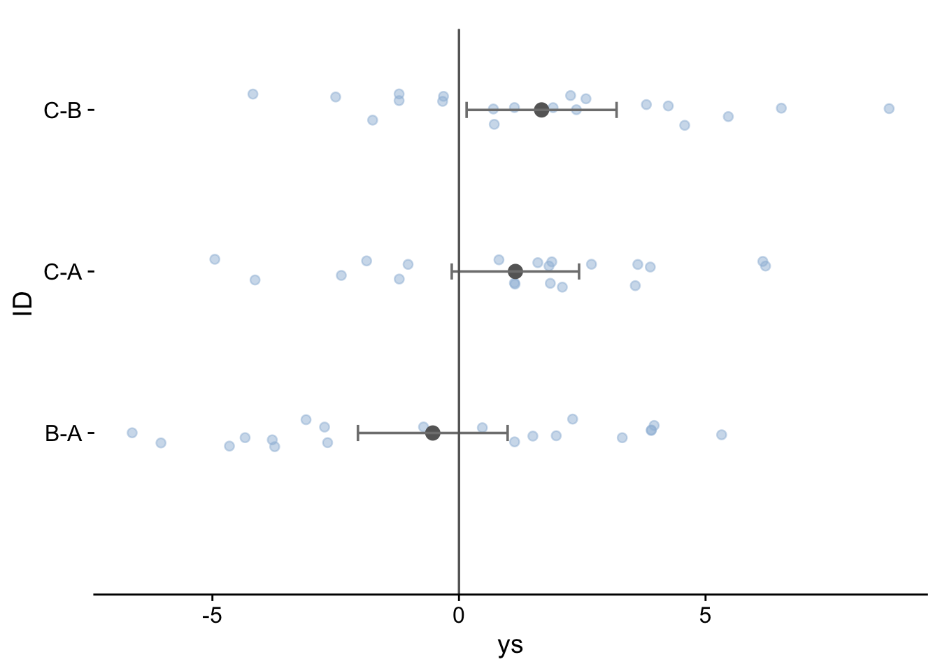
Note that where the confdence intervals straddle zero, meaning that zero i a plausible value for the respective difference, the corresponding p-value is greater than 0.05