5  Titles, labels and annotations

Often in plots one needs to use mathematical expressions, suffixes/superscripts, greeek letters or other unusual formatting.

Here we show one way of doing this, using bquote(). Over the years I have found this to be the simplest way.

5.1 Use bquote()

The four rules

• Strings – Require quotes wrapped w/ tilde separator (e.g., “my text” ~).
• Math Expressions – Unquoted & follow ?plotmath
• Numbers – Unquoted when part of math notation
• Variables – Use .() (pass in string or numeric)

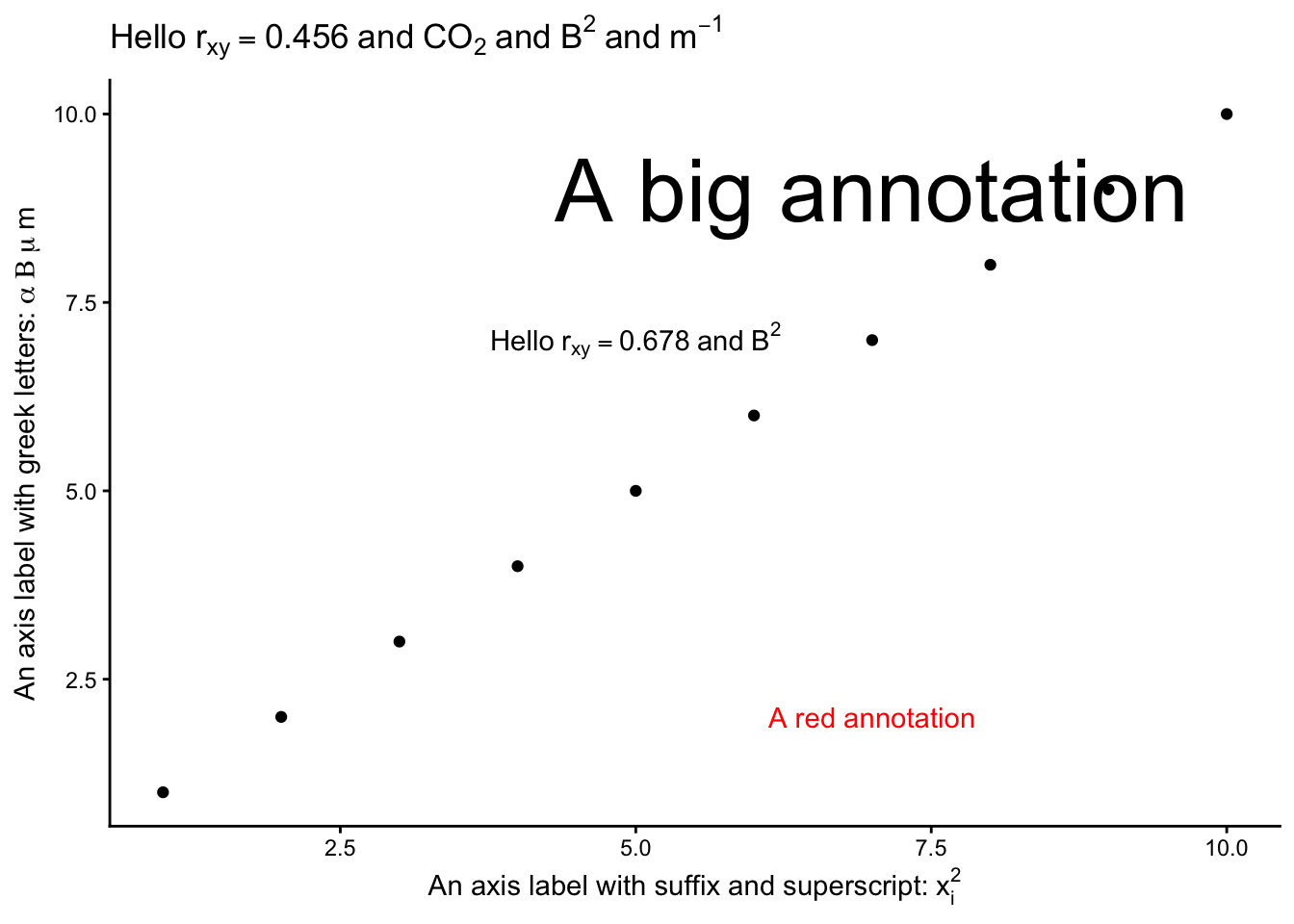
Examples of all of these are shown in the labels, title and annotations included in the plot below:

df <- tibble(x=1:10,y=1:10)
cor <- 0.456
df |>
  ggplot(aes(x=x,y=y)) +
  geom_point() +
  labs( x = bquote("An axis label with suffix and superscript:" ~ x[i]^2), 
        y = bquote("An axis label with greek letters:" ~ alpha ~ Beta ~ mu ~ m),
        title = bquote("Hello"~ r[xy] == .(cor) ~ "and" ~ CO[2] ~ "and" ~ B^2 ~ "and" ~ m^{-1})) +
  annotate(geom="text", x = 5, y = 7, label =  deparse(bquote("Hello" ~ r[xy] == 0.678 ~ "and" ~ B^2)), parse = TRUE) +
  annotate(geom="text", x = 7, y = 9, label =  bquote("A big annotation"), size = 12) +
  annotate(geom="text", x = 7, y = 2, label =  bquote("A red annotation"), colour = "red") +
  theme_classic()

5.2 ?plotmath

plotmath expressions can be used for mathematical annotation in text within plots in R when writing titles, subtitles, axis labels, legends and annotations. It works in both base R graphics and ggplot2.

In the console pane, type ?plotmath in the console pane to see the full list of options.

Some key rules are:

• subscripts: O[2] gives O₂
• superscripts: m^2 gives m², m^{-1} gives m^-1
• Lower case Greek: alpha, beta etc gives \(\alpha, \beta\) etc, so mu
• Upper case Greek: Delta, Gamma etc gives \(\Delta, \Gamma\) etc